Table of Contents
I introduce the way to sort a pivot table by summary value.
Environment
- Windows 10 Home
- Microsoft Excel 2016
Procedure to Sort by Summary Value
Here, how to sort pivot table values by summary values.
Create Pivot Table
Prepare data for the pivot table.
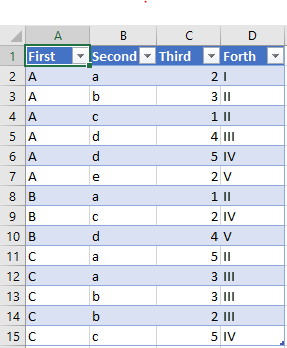
Create pivot table from the data. In the following image, there is a filter option for the latter explanation.
Sort
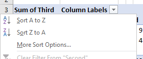
To sort rows, select the summary value cell.
Click the sort button.
To sort columns, select the summary value cell.
Click the sort button.
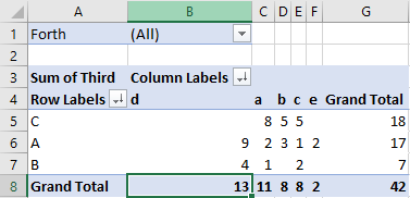
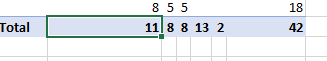
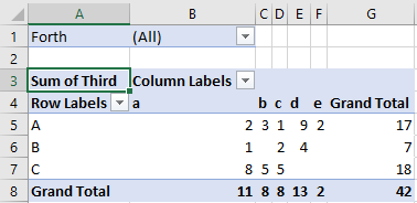
Then, the pivot table is sorted by summary values. In the following image, row and column is sorted in descending order.

Show Filtered Values Sorted by Unfiltered Summary Values
Create pivot table. After that, set up the configuration before sorting.
Set up the Sort Configuration
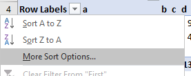
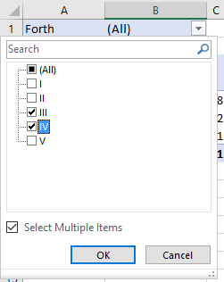
Configure row sort. Click “More Sort Option” as the following image.
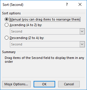
Dialog “Sort” will appear, then click “Manual“.
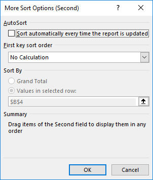
Dialog “More Sort Options” will appear, then turn off the check box “Sort automatically every time the report is updated“.
Click “OK” and close the dialogs.
Do the same for column sort configuration.
Then, sort by column and row summary values.
Set up Filtering
Add filter to the pivot table.
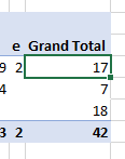
Filtered value will be shown as sorted in order of unfiltered summary value.

 Managing test specifications with Git: Creating Excel from Markdown")


