Table of Contents
Let’s introduce examples of the geometric distribution and the negative binomial distribution.
Example
We roll two dice simultaneously. Let’s call this trial A. We represent both dice showing 1 as T and any other outcome as F.
We repeat trial A until T occurs and then stop at that point. Let’s call this trial B.
In trial B, we define R as the number of times F occurs, i.e., the number of times both dice don’t show 1.
We repeat trial B \(c\) times and take the average of R, which we denote as \(X\).
Probability of \(X\)
We will write the probability of \(c, X\) as \(\textrm{P}(c, X)\).
Let’s consider the case when \(c=1\). Basically, when we roll the dice once, the probability of T appearing is \(\frac{1}{36}\), and the probability of F appearing is \(\frac{35}{36}\). Since \(\textrm{P}(1, X)\) is the probability of T appearing after \(X\) consecutive Fs, it can be expressed as:
\[ \textrm{P}(1, X) = \left(\frac{35}{36}\right)^X \frac{1}{36} \]and this is the geometric distribution with respect to \(X(=cX)\).
Let’s consider the general case when \(c\) is not 1. We roll the dice a total of \( (cX+c) \) times. The possible outcomes are combinations of \(cX\) consecutive Fs before any of the \(c\) T’s, which is the combination \({}_X \textrm{H} _{cX} (= {}_{c+cX-1} \textrm{C} _{cX} = {}_{c+cX-1} \textrm{C} _{c-1})\). In other words, it is the combination of \( (c-1) \) out of \( (c+cX-1) \) occurrences to be T. Note that for \(c \gt 1\), \(X\) can take non-integer values.
The probability is then:
\[ \textrm{P}(c, X) = {}_{c+cX-1} \textrm{C} _{c-1} \left(\frac{35}{36}\right)^{cX} \left(\frac{1}{36} \right)^c \]and this is the negative binomial distribution with respect to \(cX\). As for \(X\), it represents the distribution of averages over multiple trials \(B\), so the central limit theorem holds.
Graphing the Probability Distribution
Let’s display line graphs for \(c=1,2,5,10,20,50,100\). In Excel or LibreOffice, you can use the COMBIN function to calculate combinations and create graphs.
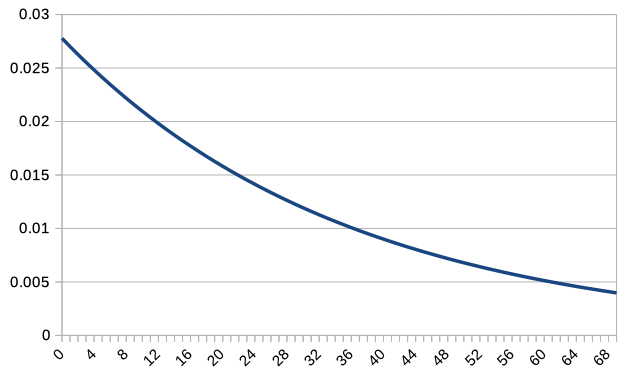
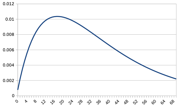
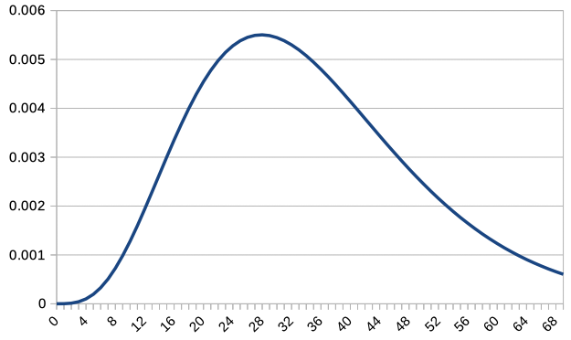
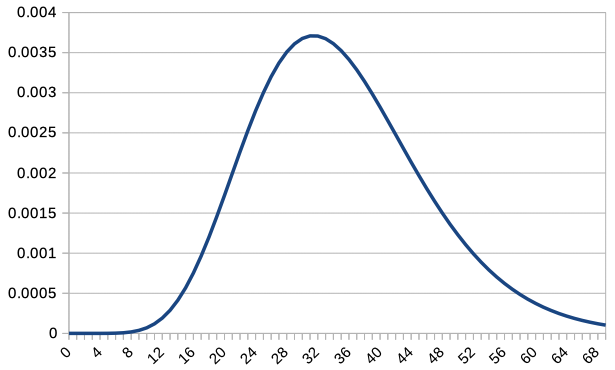
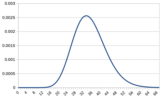
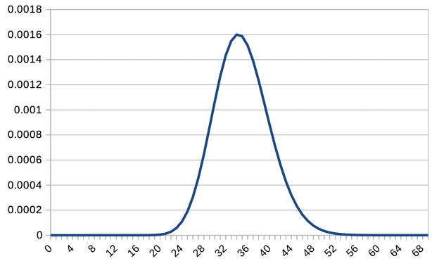
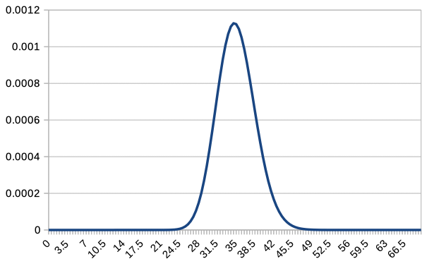
Since overlapping all graphs together makes it difficult to read, we overlay the graphs of \(c\textrm{P}(c,X)\) for \(c=1,2,5,10,20,50,100\). Note that only integer values of \(X\) are plotted, so the graph for \(c=100\) is slightly rough.
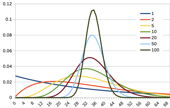
For \(c=1\), the distribution was not only asymmetrical but also decreasing to the right. However, as \(c\) increases, it becomes more similar to a normal distribution. As \(c\) increases, \(X=35\) becomes the most probable value, and the distribution changes accordingly.
Geometric Distribution
When \(c=1\), it was the geometric distribution. The geometric distribution is expressed as \(\textrm{P}(X) = p (1-p)^{X-1}\) for \(X = 1, 2, 3, \cdots\), and its \(E(X) = \frac{1}{p}\) and \(V(X) = \frac{1-p}{p^2}\).
In the above example, with \(p=\frac{1}{36}\), we can express \(\textrm{P}(X) = (1-p) \cdot p (1-p)^X\), so the expected value is \(E(X) = \frac{1-p}{p} = 35\), and the variance is \(V(X) = 35 \cdot 36\).
Negative Binomial Distribution
For \(c=1\) and the general \(c\), it was the negative binomial distribution. The negative binomial distribution for the number of failures \(X (= 0, 1, \cdots)\) before the \(k\)th success is given by \(\textrm{P}(X) = {}_{k+X-1} C_{X} p^k (1-p)^X\), and its \(E(X) = k \frac{1-p}{p}\) and \(V(X) = k \frac{q}{p^2}\).
In the above example, with \(p=\frac{1}{36}\), and considering the number of failures \(cX\) before the \(c\)th success, we can express \(\textrm{P}(cX) = {}_{c+cX-1} \textrm{C}_{cX} p^c (1-p)^{cX}\), so the expected value is \(E(cX) = c 35\), and the variance is \(V(cX) = c 35 \cdot 36\). Consequently, \(E(X)=35\), and \(V(X) = \frac{35 \cdot 36}{c}\). As observed in the graph, the expected value indeed becomes 35.
![[Simulation] the Law of Large Numbers and the Central Limit Theorem](https://improve-future.com/wp-content/uploads/2019/06/standard_normal_distribution-150x150.png "[Simulation] the Law of Large Numbers and the Central Limit Theorem")


 es un número irracional")