[Simulation] the Law of Large Numbers and the Central Limit Theorem

Table of Contents

Seeing samples, simulation in other words, is a good way to understand the concept, so I’ll explain with an example. At first, I’ll show the explanation of the law and theorem, and then I’ll provide the example.

Let’s confirm the 2 principles at first.

The Law of Large Numbers

When the sample size becomes larger, the sampling distribution of the sample average becomes more concentrated around the expectation.

The Central Limit Theorem

For all the distribution, the standardized sample average distribution converges to the standard normal distribution as the number of sample increases.

Standard Normal Distribution

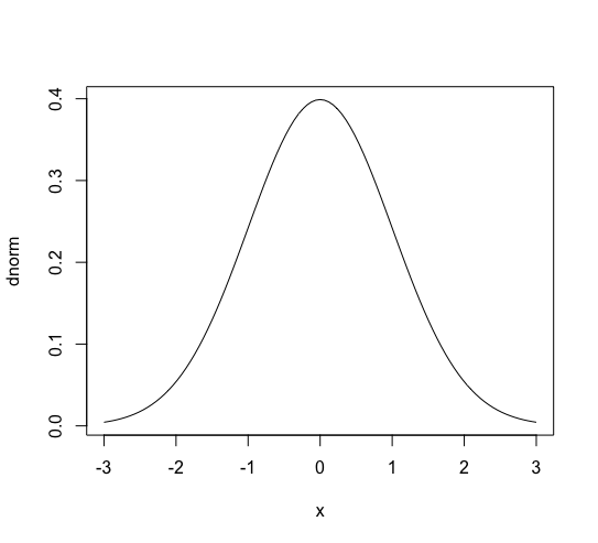
At first, standard normal distribution is a continuous distribution with density function: (f(x) = frac{1}{sqrt{2 pi} } exp left( – frac{x^2}{2}right)). Its expectation is 0 and the variance is 1. It can be plotted with plot(dnorm, xlim=c(-3, 3)) in R.

Standardization

The conversion from the variable, (x), to (frac{x – mu}{sigma} ) is the standardization. (mu) is the expectation of (x), and (sigma) is the standard deviation of (x). The distribution of (frac{x – mu}{sigma}) takes 0 for the expectation and 1 for the standard deviation.

Simulation

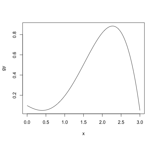
I will show the convergence simulation of distribution with a simulation here. Now, let’s think about a function (g(x) = frac{1}{10} (3-x)(x-0.4)^2 (x+1) + 0.05) for (x in [0, 3]). It can not be a density function, but it helps to build probability function. The graph of it is shown as follows.

g <- function(x) {((3 - x)*(x - 0.4)^2 *(x + 1) + 0.5)/10}
x <- (0:300)/100
gy <- g(x)
plot(x, gy, type='l')

g <- function(x) {((3 - x)*(x - 0.4)^2 *(x + 1) + 0.5)/10}

x <- (0:300)/100

gy <- g(x)

plot(x, gy, type='l')

Approximate the expectation and the variance as follows.

s <- sum(gy)
P <- function(x) { g(x) / s }
y <- P(x)
m <- sum(x * y)
v <- sum((x - m) * (x - m) * y)

s <- sum(gy)

P <- function(x) { g(x) / s }

y <- P(x)

m <- sum(x * y)

v <- sum((x - m) * (x - m) * y)

Here, x contains (0, 0.01, 0.02, cdots , 3) and gy is the values corresponding to x calculated by g. P is the probability function for x. y contains the probabilities of x calculated by P. To see the distribution of (x), type plot(x, y * 100, type='l').

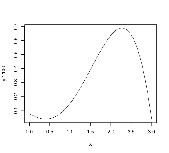
The expectation m is 1.97606, and the variance v is 0.3572804.

Now, prepare for the simulation. In the following script, pick is for picking up one x value along with the probabilities, sample_average is for calculating the average of the samples, generate_distribution is for taking sample value 100,000 times, draw_original is for drawing the occurrence graph, and draw is for drawing the sample result probability graph.

N = 100000
pick <- function() {
candidate = NA
while (TRUE) {
candidate = runif(1, 0, 3)
p = runif(1, 0, 1)
if (p < g(candidate)) break
}
candidate
}
sample_average <- function(n) {
c = 0
for (i in 1:n) { c = c + pick() }
c / n
}
generate_distribution <- function(n) {
r <- (0:300) * 0
for (i in 1:N) { r[i] = sample_average(n) }
r
}
draw <- function(n) {
X = generate_distribution(n)
plot(
table(round((X - m) / sqrt(v/n), 1)) * 10 / N,
type='l',
xlim=c(-3, 3),
ylim=c(0, 0.4),
col=rgb(1/n, 0, 1-1/n),
xlab="",
ann=FALSE,
axes=FALSE
)
}
draw_original <- function(n) {
X = generate_distribution(n)
plot(
table(round(X, 2)),
xlim=c(0, 3),
ylim=c(0, 6000),
type='l',
col=rgb(1/n, 0, 1-1/n),
xlab="",
ann=FALSE,
axes=FALSE
)
}

N = 100000

pick <- function() {

candidate = NA

while (TRUE) {

candidate = runif(1, 0, 3)

p = runif(1, 0, 1)

if (p < g(candidate)) break

}

candidate

}

sample_average <- function(n) {

c = 0

for (i in 1:n) { c = c + pick() }

c / n

}

generate_distribution <- function(n) {

r <- (0:300) * 0

for (i in 1:N) { r[i] = sample_average(n) }

}

draw <- function(n) {

X = generate_distribution(n)

plot(

table(round((X - m) / sqrt(v/n), 1)) * 10 / N,

type='l',

xlim=c(-3, 3),

ylim=c(0, 0.4),

col=rgb(1/n, 0, 1-1/n),

xlab="",

ann=FALSE,

axes=FALSE

)

}

draw_original <- function(n) {

X = generate_distribution(n)

plot(

table(round(X, 2)),

xlim=c(0, 3),

ylim=c(0, 6000),

type='l',

col=rgb(1/n, 0, 1-1/n),

xlab="",

ann=FALSE,

axes=FALSE

)

}

Simulation of the law of large numbers

The following script creates the graph of occurrences in 100,000 trials for each sampling pattern.

draw_original(1)
par(new=T)
draw_original(4)
par(new=T)
draw_original(100)
axis(side=1, at=0:3)
axis(side=2, at=(0:6) * 1000)

draw_original(1)

par(new=T)

draw_original(4)

par(new=T)

draw_original(100)

axis(side=1, at=0:3)

axis(side=2, at=(0:6) * 1000)

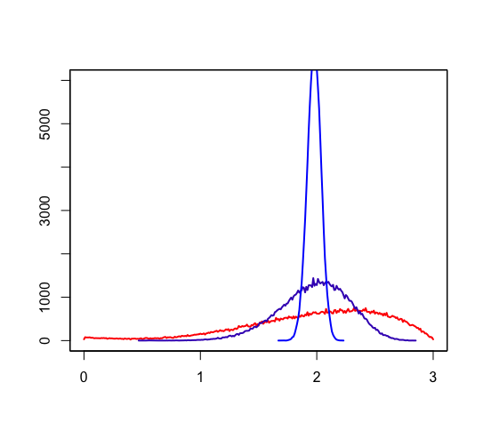
The red line is one sample occurrence. The purple one is for 4 sample average. The blue one is for 100 sample average. They show the probability around the mean, 1.97606, becomes bigger when the number of samples gets larger. It is the law of large numbers.

Simulation of the central limit theorem

Then the following script creates the image in which we can see the convergence. It is what the central limit theorem is saying.

plot(dnorm, xlim=c(-3, 3), ylim=c(0, 0.4))
par(new=T)
draw(1)
par(new=T)
draw(4)
par(new=T)
draw(100)

plot(dnorm, xlim=c(-3, 3), ylim=c(0, 0.4))

par(new=T)

draw(1)

par(new=T)

draw(4)

par(new=T)

draw(100)

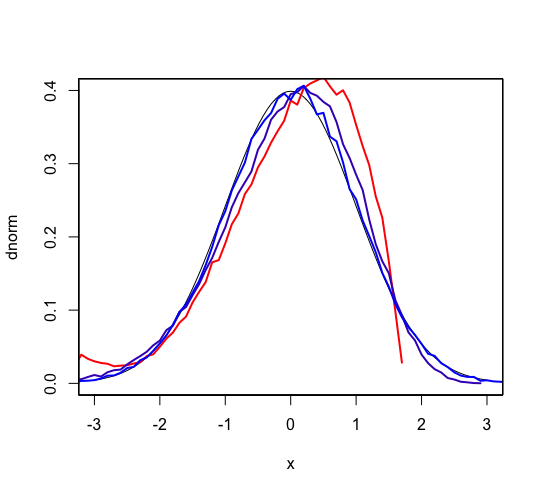
The smooth black curve is standard normal distribution. The red line is one sample trial, which doesn’t have positive value more than about 2. But the purple line, 4 samples average, has value more than 2 and it is near to standard normal distribution. The blue line, 100 samples average, is very similar to standard normal distribution. It is the central limit theorem. Theoretically, it could be the same as standard normal distribution when we increase the number of samples, at last. It means the expectation becomes near to 0 and the standard variance becomes near to 1 when the number of samples increases.