Table of Contents
Simulation is important to develop our intuitive understanding. So when the difficult content appears, try considering a sample. If there’s no handy sample, creating a sample with R is very efficient, simulation in other words.
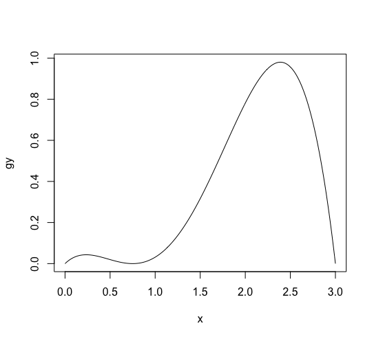
When we want to understand the law of the large number, we can also generate it virtually. Here, I will show you the simulation. Consider the function which takes (x in [0, 3)) and the value is in ([0, 1)), such as ( g(x) = frac{1}{4} x(3-x)(x-0.75)^2). ((g(x)) can’t be a density function for the random variable, because (int _0 ^1 g(x) dx neq 1). It is the probability to admit (x) value generated by randomly. It is for creating trial data.)
The following R script generates a plot of (g(x)).
|
1 2 3 4 |
g <- function(x) {x * (3 - x) * (x - 0.75) * (x - 0.75) / 4} x <- (0:300)/100 gy <- g(x) plot(x, gy, type='l') |
Suppose (x = 0, 0.01, 0.02, cdots , 2.99, 3), then P((x) = g(x) / (sum ^ {300} _ {k=0} g(100k) )).
|
1 2 3 4 5 |
s <- sum(gy) P <- function(x) { g(x) / s } y <- P(x) m <- sum(x * y) v <- sum((x - m) * (x - m) * y) |
Then m is the expectation, v is the variance. m is 2.16665, v is 0.2341004.
We can test sampling distribution with the following functions.
|
1 2 3 4 5 6 7 8 9 10 11 12 13 14 15 16 17 18 19 20 21 |
pick <- function() { candidate = NA while (TRUE) { candidate = round(runif(1, 0, 3), 2) p = runif(1, 0, 1) if (p < g(candidate)) break } candidate } sample_average <- function(n) { v = 0 for (i in 1:n) { v = v + pick() } v / n } generate_distribution <- function(n) { r <- (0:300) * 0 for (i in 1:10000) { r[i] = sample_average(n) } table(r) / 10000 } |
Then, test the law for 1 sample, 2 samples average, 5 samples average, 50 samples average and 100 samples average.
For 1 sample
|
1 |
plot(generate_distribution(1)) |
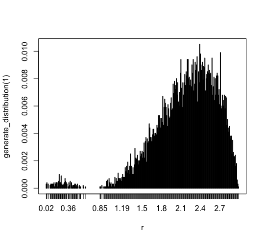
This is a test of simple one sample. It follows the function P.
For 2 samples average
|
1 |
plot(generate_distribution(2)) |
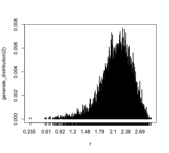
This is a trial for an average of 2 samples. Most of the data drops in [1.79, 2.69] in this trial, while the previous graph doesn’t. And the range of the data shrank. There is no data less than 0.2.
For 5 samples average
|
1 |
plot(generate_distribution(5)) |
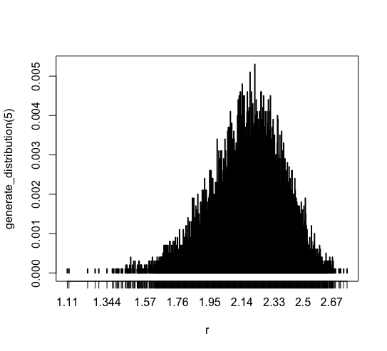
The most data drops in [1.95, 2.5]. Here, the mode looks mean value, 2.16665.
For 50 samples average
|
1 |
plot(generate_distribution(50)) |
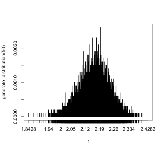
The most data drops in [2.05, 2.26].
For 100 samples average
|
1 |
plot(generate_distribution(100)) |
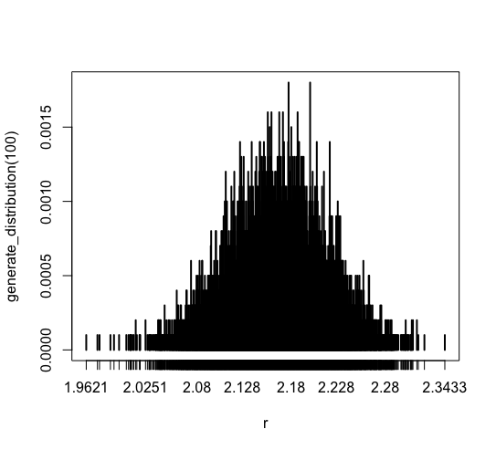
The most data drops in [2.08, 2.228], and there is no data less than 1.9621 or more than 2.3433.
I hope you figure out the Law of Large Numbers intuitively .


![[Simulation] the Law of Large Numbers and the Central Limit Theorem](https://improve-future.com/wp-content/uploads/2019/06/standard_normal_distribution-150x150.png "[Simulation] the Law of Large Numbers and the Central Limit Theorem")

</rp></ruby>町 JR東海 <ruby>下部<rp>(</rp><rt>しもべ</rt><rp>)</rp></ruby>温泉駅")
 が有理数となるような無理数 ( a ) 、 ( b ) が存在する")


